| TOP | STORE | DSSF3 | RAE | RAD | RAL | MMLIB | Support | Contact Us |
1. Main window
This window is displayed when the program starts. It consists of Menu, Toolbar, Tree view of folder, List box of measured data, and Status bar. The data saved by RA (Realtime Analyzer) and EA (Environmental Noise Analyzer) are loaded and calculated. You can see the results of calculation and export them into CSV files.
Three kinds of data as below are analyzed in SA.
| Folder color | Contents | Program which has measured and saved the data |
| Impulse Response data | "Impulse Response" function included in Realtime Analyzer | |
| ACF data | "Running ACF" function included in Realtime Analyzer | |
| Noise Measurement data | Environmental Noise Measurement System |
1-1. Menu and Command buttons
| Menu | Command | Description | Command button |
| File | Open | Opens data folder. |
|
| Not supported. | |||
| Print Preview | Not supported. | ||
| Print Setup | Not supported. | ||
| Exit | Terminates this program. | ||
| View | Toolbar | When you add a check mark, a toolbar is displayed | |
| Status Bar | When you add a check mark, a status bar is displayed. | ||
| Refresh Views | Screen is renewed in the latest condition. | ||
| Parameters | Show Parameters | Displays the analysis results of the data selected. Double click on the data list works too. | |
| Calculation | Opens the calculation condition dialog. | ||
| Output File | Calculation results are saved in the file. |
|
|
| Noise Source Template | This is available only when the folder of noise measurement is opened. Opens a dialog for setting template of noise source. |
||
| Help | Version Information | Shows version information. |
|
| Read Me | Opens Readme file. | ||
| License registration | Opens registration dialog | ||
| Buying YmecStore | Opens the purchase page (only when connected to the Internet). | ||
| Online Program Manual | Opens the online manual (only when connected to the Internet). | ||
| Technical Support | Opens the technical support page (only when connected to the Internet). | ||
| Document Q&A | Opens the Q&A page (only when connected to the Internet). | ||
| Online Update | Execute the online update (only when connected to the Internet, and available only in Version 5.x.x.x.). |
1-2. Items in the list view
< When ![]() or
or ![]() or
or ![]() is selected
in the tree view >
is selected
in the tree view >
Folders of selected kind are displayed.
< When ![]() or
or ![]() or
or ![]() is selected
in the tree view >
is selected
in the tree view >
Data which is included in the folder are displayed.
| Field | Description |
| Title | Name of measured data |
| Comment | Comment which was made when data were saved. |
| Date | Measurement date |
| Calc. | The data which has "*" mark is already calculated. Un-calculated data has no mark. |
2. Calculation of acoustic parameters
When you execute [Calculation] from the Parameters Menu, "Calculation
Conditions" dialog appears. This dialog is different between the kinds of
data (= folder) selected. Set the calculation conditions, and click [Start]
button. The calculation of acoustic parameters is done.
2-1. Impulse response data
The impulse response is analyzed in 1/1 or 1/3 octave bands. Acoustic parameters for evaluating the qualities of the sound fields and the subjective preference score are calculated according to Prof. Yoichi Ando's concert hall acoustics*.
*See Appendix for description of the theoretical background.
NEW: Calculation of ISO 3382 room acoustic parameters is available in DSSF3. (2003/12/10) See Appendix for more information.
NEW: Calculation of the MTF and STI for evaluating the speech intelligibility is available in DSSF3. (2003/06/25) See Appendix for more information.
2-2-1. Calculation conditions
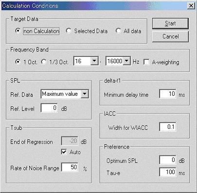
Items in the calculation conditions window
| Option | Description |
| Target Data | Select the data you want to calculate from [non Calculation], [Selected Data], and [All Data]. |
| Frequency Band | Select the frequency band (1/1 or 1/3 octave) in calculation of acoustic parameters. When [A-weighting] is checked, the A-weighted data is also calculated. |
| SPL | When "Absolute value" is selected from pop-down list of [Ref.
Data], numerical value obtained by calculation is shown as it is. In this
case, the numerical value doesn't mean the absolute sound pressure level. When "Maximum value" is selected from [Ref. Data], the maximum level data in the current folder is set as the value inputted in [Ref. Level] box. The other data in the current folder are calculated as relative levels to this data. When the other (= the data name) is selected from [Ref. Data], selected data is set as the value inputted in [Ref. Level] box. The other data in the current folder are calculated as relative levels to this data. |
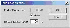
| Tsub | When the regression line of the integrated reverberation curve is calculated, the boundary of
the effective decay is set to [End of
Regression]. If [Auto] is checked, the boundary of the effective decay is
set automatically, so that the effective decay is 5dB higher than the
average noise level.
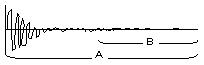
[Rate of Noise Range] is the ratio of the noise range to total impulse
response signal. (B/A)% shown in the following figure. Extra noise signal
is ignored in calculating the regression line. |
| delta-t1 | Enter the [Minimum delay time] as the delay time from the direct sound. The reflection whose delay time is shorter than this value is ignored, being regarded as the floor reflection. |
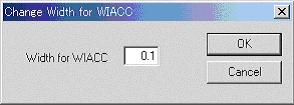
| IACC | 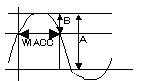 Width
for WIACC is set as (B/A)% as shown in the figure. Default value is
0.1. Width
for WIACC is set as (B/A)% as shown in the figure. Default value is
0.1. |
| Preference | Set the preferred listening level [Optimum SPL] and [Tau-e] value of the music source in the calculation of subjective preference. |
The sound data saved in the running ACF measurement in RA (monaural or stereo data) is analyzed by the autocorrelation and cross-correlation functions. Acoustical parameters representing the sound qualities (sound level, pitch, pitch strength, and reverberation), and the spatial properties (location, width of sound source, subjective diffuseness) are calculated with the high temporal resolution up to about 1 ms.
See: Introduction to the autocorrelation function
2-2-1. Calculation conditions
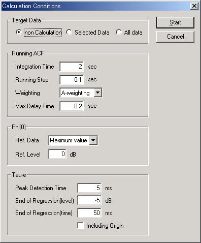
Items in the calculation conditions window
| Option | Description |
| Target Data | Choose the data you want to calculate from [non Calculation], [Selected Data], and [All Data]. |
| Running ACF | The calculation conditions of the running ACF are set up. -> More information about ACF/CCF |
| Phi(0) | When "Absolute value" is selected from pop-down list of [Ref.
Data], numerical value obtained by the calculation is shown as it is. In
this case, the numerical value doesn't mean the absolute sound pressure
level. When "Maximum value" is selected from [Ref. Data], the maximum level data in the current folder is set as the value inputted in [Ref. Level] box. The other data in the current folder are calculated as the relative value to this data. When the other (= the data name) is selected from [Ref. Data], selected data is set as the value inputted in [Ref. Level] box. The other data in the current folder are calculated as the relative value to this data. |
| Tau-e | The value of te are obtained as a
time duration (t) of 10 dB decay for a
regression line which is calculated from the initial part of
autocorrelation function (ACF) in logarithmic scale. Linear regression is
implemented by use of ACF peaks, which are extracted in every short time
duration determined as [Peak Detection Time]. When above-mentioned peak value become smaller than the value inputted in [End of Regression (level)], or when above-mentioned delay time (t) become larger than the value inputted in [End of Regression (time)], the peak detection (regression calculation) finishes. The regression calculation finishes when the condition of either the regression end level or the regression end time is met. |
Measured sound data in EA (Environmental noise Analyzer) is analyzed by the autocorrelation and cross-correlation functions. Acoustical parameters representing the sound qualities (sound level, pitch, pitch strength, and reverberation), and the spatial properties (location, width of sound source, subjective diffuseness) are calculated with the high temporal resolution up to 1 ms. In addition, template for sound identification can be edited.
See: Introduction to the autocorrelation function
2-3-1. Calculation conditions
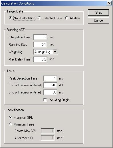
Items in the calculation conditions window
| Option | Description |
| Target Data | Choose the data you want to calculate from [non Calculation], [Selected Data], and [All Data]. |
| Running ACF | The calculation conditions of the running ACF are set up. You need to input into [Max Delay Time] enough larger than the expected te value. But, if this value is too large, calculation time becomes long. |
| Tau-e | The value of te are obtained as a
time duration (t) of 10 dB decay for a
regression line which is calculated from the initial part of
autocorrelation function (ACF) in logarithmic scale. Linear regression is
implemented by use of ACF peaks, which are extracted in every short time
duration determined as [Peak Detection Time]. When above-mentioned peak value become smaller than the value inputted in [End of Regression (level)], or when above-mentioned delay time (t) become larger than the value inputted in [End of Regression (time)], the peak detection (regression calculation) finishes. The regression calculation finishes when the condition of either the regression end level or the regression end time is met. |
| Identification | It is possible to choose the data to use for identification from maximum value of F(0) or minimum value of te. When the (Tau-e)min is chosen, user sets what steps before and after F(0)max should be included in the target data. "Step" is the calculation interval. The ACF/CCF parameters are calculated in every calculation step. |
3. Display of calculated acoustic parameters
Select the data and then execute [Show Parameters] from Parameters menu (or double click on the data), the acoustic parameter window is displayed, where you can see calculated acoustic parameters. Corresponding to three kinds of data (= Impulse response data, ACF data, and Noise measurement data), the different window appears.
3-1-1. Data information display and buttons
3-1-1. Data information display and buttons
| Field | Description |
| Folder Information | Information about the folder which includes the data displayed on the screen are indicated. |
| Data | The measurement conditions of the data displayed on the screen are indicated. |
| Calculation Conditions | The calculation conditions of the data displayed on the screen are indicated. |
| Acoustic Parameters | List of the acoustic parameters which are calculated from impulse response data are indicated for each octave band frequencies. |
| Exit | Closes this window. |
| Select Data | A main window is displayed, where you can choose other data. |
| Previous | Previous data ( = the data located one line up on the main window) is displayed. |
| Next | Next data ( = the data located one line down on the main window) is displayed. |
Top of the impulse response data
| Parameter | Description | Unit |
| Freq. | Frequency. All(F): Full range, All(A): A-weighted, Others: Center frequency of band-limited noise. | Hz |
| SPL-LR | The average listening level of both channels. | dB |
| SPL-L | Left channel's Listening level. | dB |
| SPL-R | Right channel's Listening level. | dB |
| dt1-LR | The average of initial time delay gap between the direct sound and the initial reflections (Dt1)of both channels: The time after direct sound arrives until the initial reflections arrive. As for Dt1, the calculation is done for only full range. | ms |
| dt1-L | Left channel's Dt1. | ms |
| dt1-R | Right channel's Dt1. | ms |
| A-LR | The average of total amplitude of reflections of both channels. | dB |
| A-L | Left channel's total amplitude of reflections. | dB |
| A-R | Right channel's total amplitude of reflections. | dB |
| Tsub-LR | The average reverberation time of both channels: Time for reducing the subsequent reverberation time by 60dB. | sec |
| Tsub-L | Left channel's reverberation time. | sec |
| Tsub-R | Right channel's reverberation time. | sec |
| IACC | Degree of the inter-aural cross-correlation function between sound signals arriving at both ears. This parameter is closely related to the subjective diffuseness of the sound field. | |
| TIACC | The delay time of the cross-correlation function. This parameter represents the horizontal direction of a sound source. | ms |
| WIACC | The width of the cross-correlation function. This parameter represents the apparent source width (ASW). | ms |
| S | Subjective preference score. |
Top of the impulse response data
There are seven tabs which have different contents in the graph area. When you click on the frequency field ("Freq.") of the acoustic parameters table, the graphs of each octave band frequency can be seen.
| Tab | Description |
| Impulse response | Impulse responses in two channels are displayed. Direct and first reflective sounds can be specified by cursors. |
| Reverberation | Echo time pattern (impulse response), decay curve, and Schroeder integration curve are displayed. |
| Cross correlation | Cross-correlation function between two channels is displayed. |
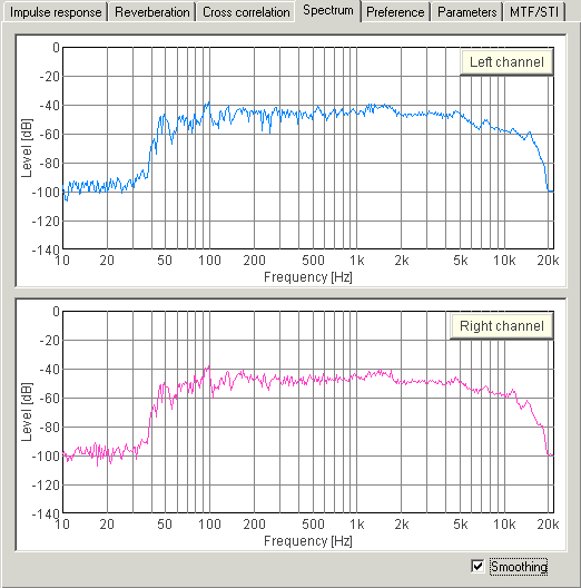
| Spectrum | Power spectrum is displayed. |
| Preference | Preference curve is displayed. |
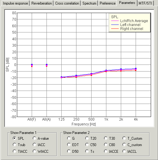
| Parameters | Frequency characteristics of the acoustic parameters are displayed. |
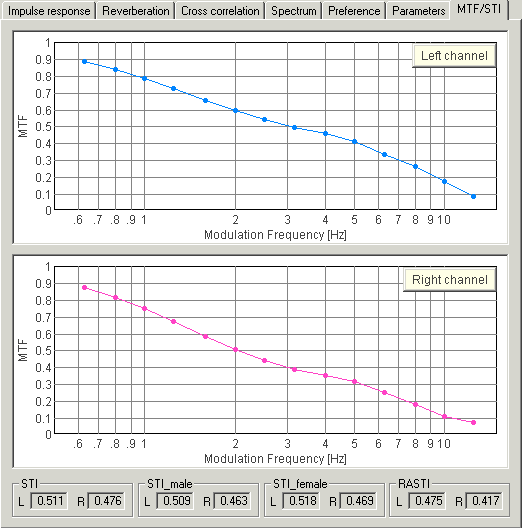
| MTF/STI | MTF (Modulation Transfer Function) and STI (Speech Transmission Index) are displayed. |
Operation in each graph tab is described below.
Top of the impulse response data
Impulse response waveforms at both channels are displayed. The display range
can be adjusted by [All], [Zoom Out], [Zoom In] button, and by moving the
scrollbar between two graphs or by dragging the graph directly.
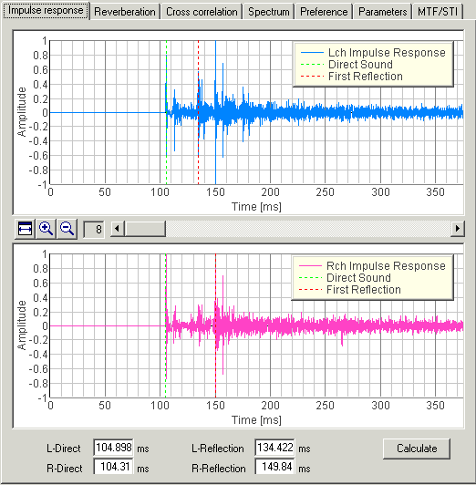
Arrival times of the direct sound and the first reflection can be modified by dragging the dashed lines (Green = direct sound, Red = first reflection) on the graphs or by inputting values to the textboxes under the graphs. Clicking [Calculate] button after this alteration, the acoustic parameters are re-calculated.
Echo time pattern (impulse response), energy decay curve (squared impulse response in dB scale), and Schroeder integration curve (backward integrated squared impulse response) are displayed. Display range can be changed by [All], [Zoom Out], [Zoom In] button, and by moving the scrollbar or by dragging the graph directly.
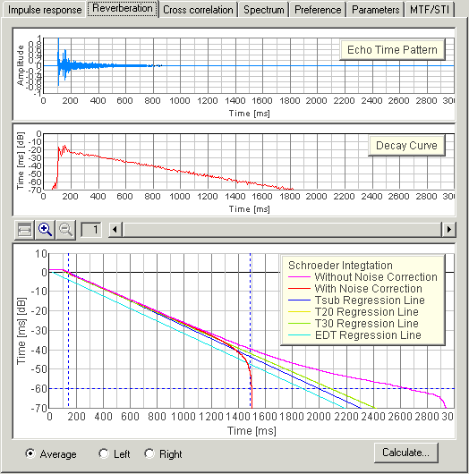
You can select the displayed channel from the radio button under the graphs. When [Average] is checked, average of both channels is displayed. Similarly, [Left] and [Right] channel can be selected.
In the Schroeder Integration display, the regression lines for measuring the reverberation times are also shown. By clicking [Calculate] button, the following dialog appears. You can change the calculation condition of Tsub and calculate it again.
The cross-correlation function is displayed within the range between -1 and +1 ms. The delay time of the maximum peak indicates the azimuth of the sound source, and its amplitude indicates the degree of correlation between two channels that is corresponding to the subjective diffuseness or spaciousness of the sound field. The width of the maximum peak is called WIACC, and represents the apparent source width.
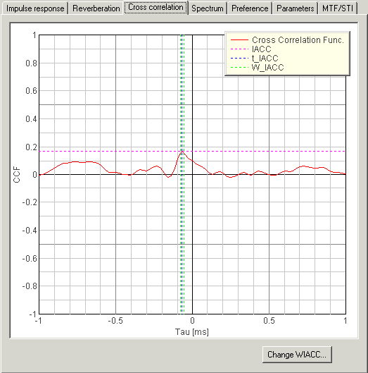
By clicking [Change WIACC] button, the following dialog appears. You can change calculation conditions of WIACC and calculate it again.
Power spectrum of the impulse response is displayed. This is the transfer function between the sound source and the microphone. If [Smoothing] box is checked, the spectra become easy to see as the small fluctuation is averaged.
Based on the Ando's theory, the subjective preference is calculated using four orthogonal parameters (SPL, Dt, Tsub, and IACC). S1- S4 are preferences scores of those parameters. Total preference SS is calculated from the summation of S1 to S4. The curve represents the preference score for different music te. The optimal SPL and the te of the music should be set before calculation.
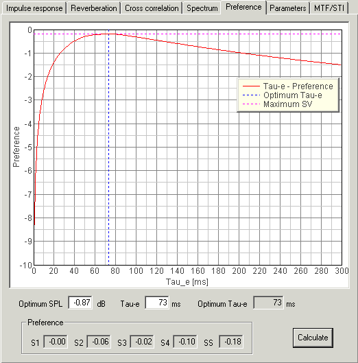
If you click [Calculate] button after modifying [Optimum SPL] and [Tau-e], the preference values are re-calculated and the graph and the numerical values (S1-S4, SS) are refreshed.
Ando's six parameters and ISO 3382 room acoustic parameters calculated from the impulse response are displayed for each frequency band. The parameter chosen from [Show Parameter] is displayed.
For evaluating the speech intelligibility in the room, MTF (Modulation Transfer Function), STI (Speech Transmission Index), and RASTI (Rapid STI) are displayed.
See appendix: Calculation of the speech transmission index
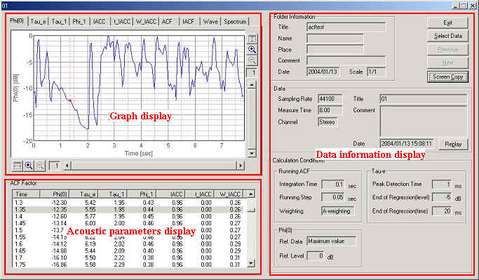
3-2-1. Data information display and buttons
3-2-2. Acoustic parameters display
3-2-1. Data information display and buttons
| Fields | Description |
| Folder Information | Information about the folder which includes the data displayed on the screen are indicated. |
| Data | The measurement conditions of the data displayed on the screen are indicated. |
| Calculation Conditions | The calculation conditions of the data displayed on the screen are indicated. |
| ACF Factor | Four ACF factors for each running step are indicated. A factor which is selected here will be expressed as a red point in the upper graph. |
| Exit | Closes this window. |
| Select Data | A main window is displayed, where you can choose other data. |
| Previous | Previous data ( = the data located one line up on the main window) is displayed. |
| Next | Next data ( = the data located one line down on the main window) is displayed. |
3-2-2. Acoustic parameters display
| Field | Description | Unit |
| Time | Measurement time. | s |
| ACF parameters (calculated for the left channel input) | ||
| Φ(0) | Signal energy. It represents the sound pressure level when the sound was measured by the calibrated microphones. | dB |
| τe | The effective duration of the ACF. It represents the reverberation components contained in the signal. | ms |
| τ1 | The time delay of the first peak in the ACF. The reciprocal of this value represents the fundamental frequency of the signal. | ms |
| φ1 | The amplitude of the first peak in the ACF. It represents the strength of the periodicity. | - |
| CCF parameters | ||
| IACC | The degree of the cross-correlation between channels. When the sound was measured by using the dummy head or microphones attached to the real head, it represents the subjective diffuseness of the sound field. | - |
| τIACC | The time delay of the cross-correlation. When the sound was measured by using the dummy head or microphones attached to the real head, it represents the horizontal direction of the sound field. | ms |
| WIACC | The width of the cross-correlation function. When the sound was measured by using the dummy head or microphones attached to the real head, it represents the apparent width of sound source (it becomes high values when the signal contains lower frequency components). | ms |
The graph display consists of 11 tabs (in the case of monaural measurement, it decreases to seven). The ACF/CCF parameters are displayed as a function of time. The ACF and CCF are displayed as a function of t. Selected data in the parameters table is displayed as in the figures below.

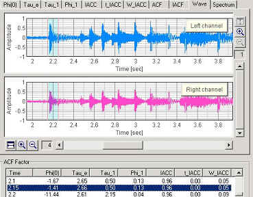
In each parameter graph, horizontal axis (time) and vertical axis (parameter value) can be zoomed in to see a specific area in detail. Once a zoom button is clicked, the displayed area can be moved to any direction freely by dragging a graph. By clicking the "Screen Copy" button, those graphs are saved as a picture file (png format).
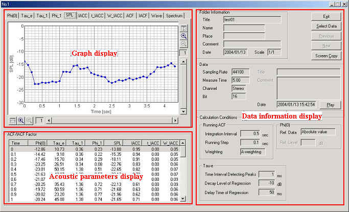
3-3-1. Data information display and buttons
3-3-2. Acoustic parameters display
3-3-1. Data information display and buttons
| Field | Description |
| Folder Information | Information about the folder which includes the data displayed on the screen are indicated. |
| Data | The measurement conditions of the data displayed on the screen are indicated. |
| Calculation Conditions | The calculation conditions of the data displayed on the screen are indicated. |
| ACF/IACF Factor | ACF factor and IACF factor for each running step are indicated. A factor which is selected here will be expressed as a red point in the upper graph. |
| Exit | Closes this window. |
| Select Data | A main window is displayed, where you can choose other data. |
| Previous | Previous data ( = the data located one line up on the main window) is displayed. |
| Next | Next data ( = the data located one line down on the main window) is displayed. |
Top of the noise measurement data
3-3-2. Acoustic parameters display
| Field | Description | Unit |
| Time | Measurement time. | s |
| ACF parameters (calculated for the left channel input) | ||
| Φ(0) | Signal energy. It represents the sound pressure level when the sound was measured by the calibrated microphones. | dB |
| τe | The effective duration of the ACF. It represents the reverberation components contained in the signal. | ms |
| τ1 | The time delay of the first peak in the ACF. The reciprocal of this value represents the fundamental frequency of the signal. | ms |
| φ1 | The amplitude of the first peak in the ACF. It represents the strength of the periodicity. | - |
| CCF parameters | ||
| IACC | The degree of the cross-correlation between channels. When the sound was measured by using the dummy head or microphones attached to the real head, it represents the subjective diffuseness of the sound field. | - |
| τIACC | The time delay of the cross-correlation. When the sound was measured by using the dummy head or microphones attached to the real head, it represents the horizontal direction of the sound field. | ms |
| WIACC | The width of the cross-correlation function. When the sound was measured by using the dummy head or microphones attached to the real head, it represents the apparent width of sound source (it becomes high values when the signal contains lower frequency components). | ms |
Top of the noise measurement data
The graph display consists of 11 tabs (in the case of monaural measurement, it decreases to seven). The ACF/CCF parameters are displayed as a function of time. The graph images of ACF and CCF are displayed as a function of t. Selected data in the parameters table is displayed as in the figures below.
In each parameter graph, horizontal axis (time) and vertical axis (parameter value) can be zoomed in to see a specific area in detail. Once a zoom button is clicked, the displayed area can be moved to any direction freely by dragging a graph. By clicking the "Screen Copy" button, those graphs are saved as a picture file (png format).
Top of the noise measurement data
4. Output of the calculated acoustic parameters
You can output your calculation results in a file by using [Output File] from
[Parameters] menu.
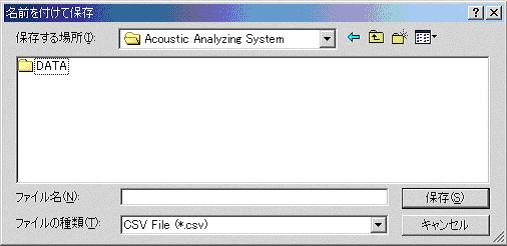
In case of the .csv filename extension, the data is outputted in the CSV file
format and in case of the .txt filename extension, the data is outputted in the
text file format.
5. Noise source template dialog
Noise source template to identify the noise is set. This dialog is available only when the noise measurement folder is open.
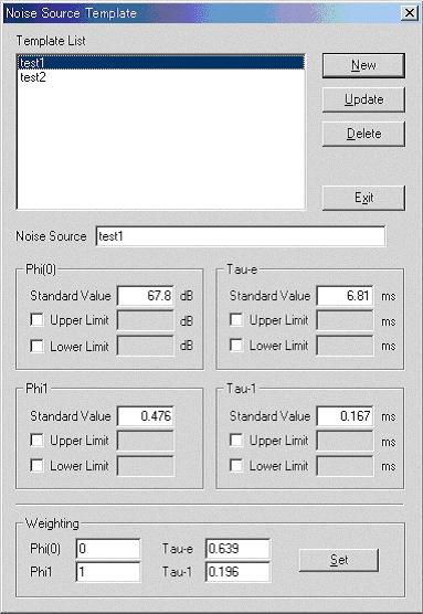
Items for setting
| Field | Description |
| Template List | Registered noise source templates are shown. |
| Noise Source | Name of the noise source. |
| Phi(0) | Input the standard value (average value), the upper limit, the lower
limit of F(0) of target noise source. If you want to set the upper limit
and the lower limit, check each box. The data which exceed the established range are not applied to this template. |
| Tau-e | Input in the same way as above-stated. |
| Phi1 | Input in the same way as above-stated. |
| Tau-1 | Input in the same way as above-stated. |
| Weighting | Weighting coefficient of each factor which is used for identification is
set. The more large the value is, the more its factor contributes to identification. |
| Button Name | Description |
| New | Creates new noise source template. |
| Update | Renews the noise source template which is selected on the list. |
| Delete | Deletes the noise source template which is selected on the list. |
| Exit | Closes this dialog. |
Measurement data of Realtime Analyzer, Sound Analyzer, and Environmental noise Analyzer, and the related data such as the microphone calibration data, the inverse filter, and the noise source template, are stored in the common database. In this section, it is explained how to manage the measurement data and delete the stored data.
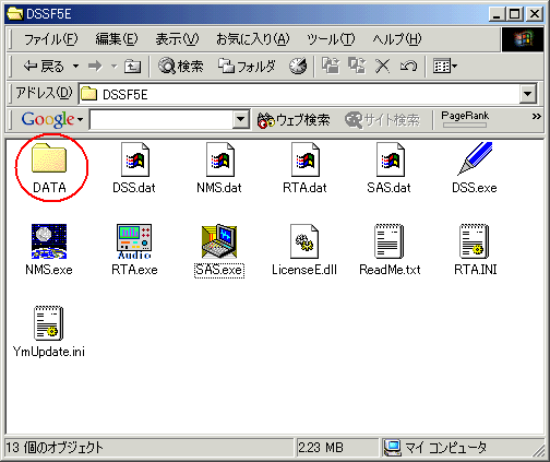
All of the measured data and the microphone calibration data are stored in the DATA folder in the program folder (DSSF5E). The database of DSSF3 is 64-bit, and the maximum data size of 2000 GB can be stored. The database of RAE, RAD, and MMLIB is still 32-bit at the time of default installation, but once you install the DSSF3, these software can also use the 64-bit database.
On-line update of the program never erase the data you have stored in the DATA folder. However, when you "re-install" the program, all the data is erased, because the sample data overwrites the existing data. To protect the already stored data, you have to backup the existing data before reinstallation. How to backup data is as below.
This backup operation enables you to use the existing data after reinstallation.
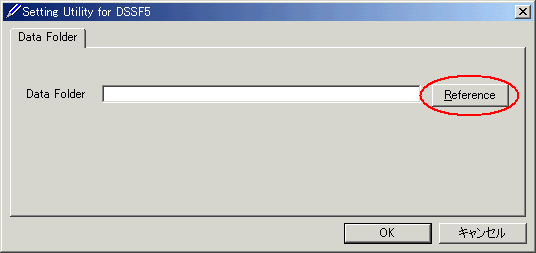
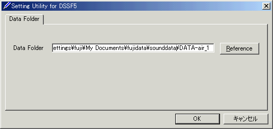
New function of DSSF3 version 5: Setting Utility to specify the data folder
In the RA series (RAD and RAE), measurement data is always stored in the "DATA" folder. To backup the data, this DATA folder has to be moved to the other location or renamed every time. But in the latest version of DSSF3, this problem has been solved. If you are using the DSSF3 version 5, you can specify the data folder by using the setting utility (DSS.exe). Wherever the measurement data is saved (even in the other computer on the network), DSSF3 can use this data. By this function, management of the measurement data becomes much easier.
1. Run the DSS.exe and click the Reference button.
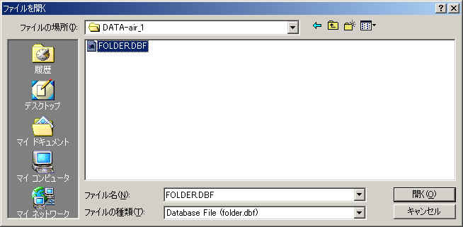
2. Specify the measurement data folder, then the file FOLDER.DBF is displayed. Select this file and click the Open button.
3. Click the OK button. Now the data in the specified folder is used by the DSSF3.
6-3. How to delete stored data
As described above, all of the measurement data is stored in the DATA folder. If you want to clear all the data, delete the DATA folder. After this operation, the new DATA folder is created so that you can start the measurement again. How to delete specific data is different for the type of data. Data type is shown in the left column of the main window of Sound Analyzer. As shown below, there are three types of data: Impulse response, Running ACF, and Noise Measurement.
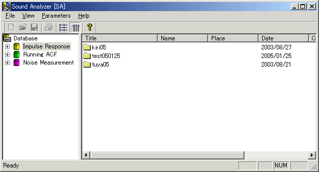
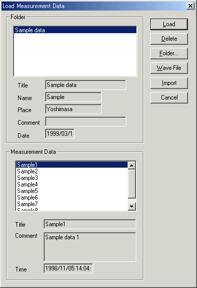
1. Delete Impulse Response data
Open the Impulse Response window from the Realtime Analyzer. Click "Load" button. Folder and Measurement data are displayed. To delete a specific data in a specific folder, select the folder and select the data, then click the "Delete" button. To delete a whole folder, select the folder and click the "Delete" button.
2. Delete Running ACF data
Open the Running ACF window from the Realtime Analyzer. The following procedure is same as above.
3) Delete Noise Measurement data
There is no way to delete the specific data of this type. Data is stored in the files "NMS.BIN" and "NMS.DBF" in the DATA folder in the program folder. If you don't need whole data, you can delete these two files. But if you need some of data, you have to backup these files to the another hard disk.
| Y Store. |
| TOP | STORE | DSSF3 | RAE | RAD | RAL | MMLIB | Support | Contact Us |
If you have questions or comments about this
page,
feel free to contact us by email ymec@ymec.com
or by online
inquiry form.