| TOP | STORE | DSSF3 | MMLIB | Support | Contact Us |
The spectrum analysis is the way to analyze signal in the frequency domain. On the other hand, the Auto-Correlation Function and the Cross-Correlation Function are the methods to analyze signal in the time domain.
The correlation function that shows the similarity of the signal itself is especially called the auto-correlation function (ACF). The ACF is a useful tool in the signal analysis because it can be used to detect the periodicity of the signal. It has been found that the ACF is strongly related to the subjective evaluation of sound. For example, in a concert hall, the most preferred reverberation time and the delay time of the reflections are calculated from the ACF of music to be performed.
The cross-correlation function (CCF) is used to investigate the similarity of two time series signals. CCF is expressed as a function of t (delay time) to show the time change of the similarity. By searching the delay time at which the cross correlation is the maximum, signal detection in noise or prediction of the transmission path of signal are possible.
The parameters extracted from the ACF and the IACF (inter-aural cross correlation function: the special case of the CCF measured by microphones at the ear positions) have a close relation with the primary sensations of sound, such as loudness, pitch, pitch strength, sound location, etc. Such features can be used for the sound quality analysis of noise, diagnosis of motor and fan, medical diagnosis of auscultation sound, or the analysis of voice quality.
more info: About the correlation function
2. Features of RA's running ACF measurement system
The Realtime Analyzer works as a data recorder for the Sound Analyzer, in which time histories of sound properties will be analyzed at a high time resolution. Tonal quality of sound, pitch and pitch strength, sound level, spatial information of sound source can be analyzed from the detailed acoustical parameters.
*1 ACF/CCF measurement system has been developed assuming the
post analysis by SA. We recommend RAD, RAE, DSSF3 Full-system version, or DSSF3
environmental noise, to use this function. See the
function list for more information about the available functions in each
version of the program.
*2 These functions are available only in the latest version of RA (Ver. 5.0 or
later). Check the version of your software. Please contact to
ymec@ymec.com
if you want the version up.
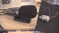
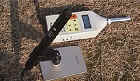
As shown in the figure below, connect the microphones and the amplifier to the soundcard. To measure the CCF, two microphones are needed. If you use only one microphone, connect it to the left channel.
Select the input device and the soundcard in the main window of RA. The Input device selection and volume control in RA is interlocked with the Windows recording control.
Check the Peak Level Monitor and adjust the input volume so that the peak level becomes between -10 and -5 dB. If the peak level reaches 0dB, the input signal might be distorted. See the operation guide to know more about volume setting.
3-3. Configuration of the measurement conditions
Before performing the measurement, check the measurement settings and the display settings. The important settings are explained below. See the reference manual for other items.
 |
Sampling Rate |
|
Time |
|
|
Channels |
|
|
Integration Time |
|
|
Running Step |
|
| Freq. Weighting Select the frequency weighting filter. Usually, select Flat or A-weighting. A-weighting filter roughly simulates the sensitivity curve of human ear, that attenuates low and high frequencies. |
3-4. Performing the measurement
Start the measurement
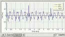
Click the start button to perform a measurement. Input signal is recorded for the specified measurement time. Calculated ACF and the input waveform is displayed in real time.
Changing the display settings
After the measurement is finished, display settings can be changed. Click the Redraw button to display the new results.
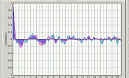
Waveform display and replay sound
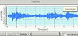
A temporal waveform of the recorded sound is displayed below the ACF graph. Horizontal axis is time [s] and the vertical axis represents the amplitude. When the input level is small, check the Normalization box. Normalized waveform between ±1 will be displayed for clarity. Click the Replay button to listen to the recorded sound.
Editing the input wave
Only the useful part of the signal can be saved by using the editing function. Right click the waveform display and drag the mouse. Then the selected area is displayed in blue. Click the Cut button to remain the selected area and cut out the non selected area.
3-5. Loading the measurement data, wav file, importing the database
Click the Load button to open the "Load Measurement Data" dialog. Saved data is displayed on the dialog. Select the data and click the Load button.
To open the wav file, click the "Wave File" button. In RAD and RAE, loadable wav files are with the resolution of 16 bit. In DSSF3, wav files with 8, 16, and 32 bit can be loaded.
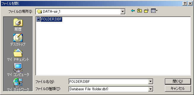
Click the Import button to load the measurement database. When selecting the folder in which the measurement data is saved, a file "FOLDER.DBF" is displayed as shown below. Select this file and click the Open button. By this operation, the previous measurement data is added to the current database. It is useful for comparison of different measurements at a time.
3-6. Saving the measurement data
Click the "Save" button on the Running ACF window, then the "Save Measurement Data" dialog opens. To save data, 1) enter the title and comment on the data, 2) select the folder, and 3) click the "Save" button. Once the data is saved, the acoustical parameters can be calculated by using SA (Sound Analyzer)*. To save sound as a wav format, click the Wave File button.
*See the SA program manual for how to analyze the ACF / CCF data.
When you make a new folder, click the "Folder..." button on the "Save Measurement Data" dialog. Folder Management dialog opens as in the figure below. Enter the title of the folder and click "New" button.
Click "Load" button. Folder and Measurement data are displayed. To delete a
specific data in a specific folder, 1) select the folder and 2) select the data,
3) then click the "Delete" button.
To delete a whole folder, 1) select the folder and 2) click the "Delete" button.
Measurement data of Realtime Analyzer, Sound Analyzer, and Environmental noise Analyzer, and the related data such as the microphone calibration data, the inverse filter, and the noise source template, are stored in the common database. Below, it is explained how to manage the measurement data and delete the stored data.
All of the measured data and the microphone calibration data are stored in the DATA folder in the program folder (e.g. DSSF5E). The database of DSSF3 is 64-bit, and the maximum data size of 2000 GB can be stored. The database of RAE, RAD, and MMLIB is still 32-bit at the time of default installation, but once you install the DSSF3, these software can also use the 64-bit database.
On-line update of the program never erase the data you have stored in the DATA folder. However, when you "re-install" the program, all the data is erased, because the sample data overwrites the existing data. To protect the already stored data, you have to backup the existing data before reinstallation. How to backup data is as below.
This backup operation enables you to use the existing data after reinstallation.
New function of DSSF3 version 5: Setting Utility to specify the data folder
In the RA series (RAD and RAE), measurement data is always stored in the "DATA" folder. To backup the data, this DATA folder has to be moved to the other location or renamed every time. But in DSSF3, this problem has been solved. If you are using the DSSF3 version 5, you can specify the data folder by using the setting utility (DSS.exe). Wherever the measurement data is saved (even in the other computer on the network), DSSF3 can use this data. By this function, management of the measurement data becomes much easier.
1. Run the DSS.exe and click the Reference button.
2. Specify the measurement data folder, then the file FOLDER.DBF is displayed. Select this file and click the Open button.
3. Click the OK button. Now the data in the specified folder is used by the DSSF3.
Measurement examples by RA can be seen in the Introduction to Sound Measurement. Relevant application notes are the following.
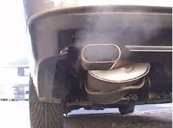
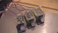
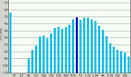
Measurement of rotational speed of a motor
| Y Store. |
| TOP | STORE | DSSF3 | MMLIB | Support | Contact Us |
If you have questions or comments about this
page,
feel free to contact us by email ymec@ymec.com
or by online
inquiry form.