| Japanese | English |
Engine's exhaust note is very important for maintenance and tuning of the race car, because the sound directly reflects the condition and the performance of engines. Some people can diagnose the performance of engines only by hearing its operation sound. I believe that the similar task can be achieved by analyzing sound's characteristics.
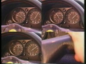
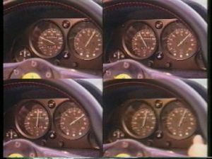
In this series of the measurement report, I analyzed the engine sound recordings of a movie. The movie was dubbed to a digital video tape, and transferred to the PC via iLINK connection. The video camera I used is SONY DCR-PC3-NTSC, and the PC is SONY VAIO PCG-R505R/DK. Pictures in the following pages are taken from the screen. Captured sounds were saved as wav files, so that I can analyze them repeatedly.

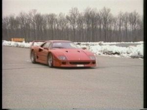
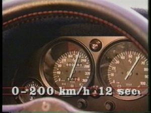
This time is a measurement of the engine sound during standing-start acceleration of F40. It reaches from 0-200 km/h by 12 seconds.
Sound file: ![]() car4.wav (44.1kHz / Stereo / 15sec / 2,585KB)
car4.wav (44.1kHz / Stereo / 15sec / 2,585KB)
Right-click the link to download the sound file. Realtime analyzer (RA) of DSSF3 has a function to load and analyze the wav files.
Start RA and set the "Input Device" as WAVE.
Open the Recorder and click the "Load" button. The waveform of the sound is displayed as below. The length of the sound is 15 seconds.
Open the FFT analyzer's spectrum view. Set the parameters as in the following figure. By clicking the "Start" button, the loaded wav file is played and the analysis is started.
Below is a screen copy at 2 seconds. You can see that several peaks are dominant. The lowest peak is the fundamental frequency (59.2 Hz), and harmonics are multiple integers of it (120, 180, 240, and so on). The rotation speed of the engine can be calculated from the fundamental frequency as described in Automobile noise analysis 1. The power spectrum is a convenient analysis method to see the frequency contents of sound and vibration. But it may be difficult to follow up the frequency peaks because the spectrum changes rapidly. To see the time-varying spectra, spectrogram is a more useful display method.
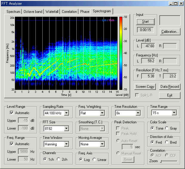
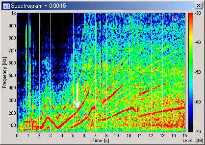
Open the FFT analyzer's spectrogram view. Set the "Time Range" as 15 s (length of sound), "Color Scale" as "Tone", and "Direction of Axis" as "Fwd", and start the measurement. In the spectrogram, the energy at a given time and frequency is displayed as a color map in a two dimensional diagram. Resolutions of frequency and time are displayed in the right of the graph (F: 5.38 Hz, T: 23.2 ms). Those are decided by the settings of the sampling rate (44.1 kHz), FFT size (8192), and time resolution (x8).
We can see the strong energy components (red or yellow curves) are temporally varying. To see these components in more detail, let's change the display range.
Level range and Freq. range were changed. Freq. Axis was also changed from Log to Linear.
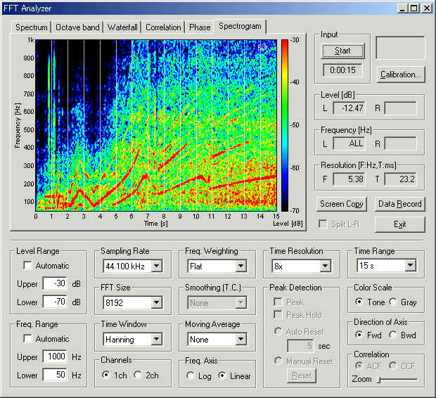
Now, the change of sound can be seen more clearly. It can be interpreted as follows:
Next, the running ACF (Auto-Correlation Function) analysis was applied to the same sound. Running ACF is the time domain analysis that is capable of detecting the periodic events better than the frequency analysis. This is the reason why we apply this method to the analysis of sounds emitted from motor, car engine, and other equipments and machinery. Of course, the autocorrelation is a good analysis method for musical instruments and voices, because most sounds are periodic or quasi-periodic in nature.
Open the "Running ACF" window from the Realtime Analyzer, and load the wav file. Step by step instruction of the ACF analysis is here. Save data into the measurement database and analyze it by the Sound Analyzer (SA).
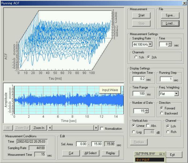
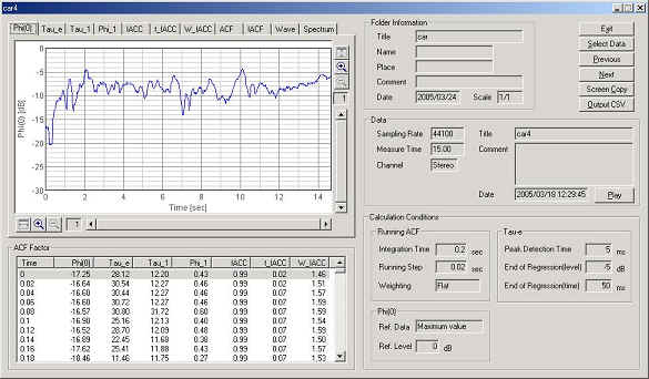
Main window of SA. Saved data is displayed in the list. Data that is not yet analyzed is indicated as a blue icon. To analyze data, select Parameters > Calculation, from the menu bar.
Calculation conditions were set as follows. Integration time (analysis data length) was set to 0.2 sec, and running step (calculation interval) was set to 0.02 sec. These values are comparable to those of the spectrogram (i.e. in the spectrogram, analysis data length is: FFT size (8192) / Sampling rate (44100) = 0.185 s, and calculation interval is Resolution [T]: 23.2 ms = 0.0232 s).
After the calculation is completed, the data icon turns to red. Double click the data name to see the results. Analysis results are displayed in several graphs and tables of the acoustic parameters. Below (Phi(0)) is the time course of the change in the relative sound level.
Next is the result of Tau_1 [ms], the delay time of the first peak in the ACF. Roughly speaking, it corresponds to the fundamental frequency as shown in the spectrogram. Difference is that Tau_1 is represented in time, that is, 1000 / Tau_1 [ms]= Frequency [Hz]. For example, 10 ms of Tau_1 means the fundamental frequency of 100 Hz. So, the upside down of Tau_1 graph looks like the red curve in the spectrogram.
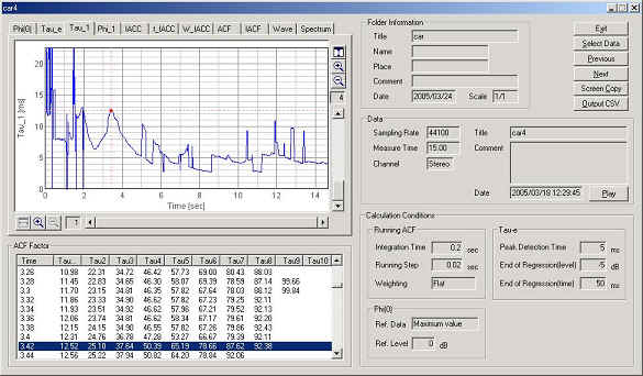
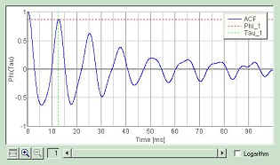
Below is the ACF waveform at 3.42 s. First peak is found at 12.5 ms, meaning its frequency is 80 Hz.
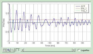
Next is the ACF at 5.3 s. The first peak is at 4.65 ms (215 Hz). Note that the second peak is at 8.87 ms (112 Hz), and is higher than the first peak. It means that at this moment, the sound consists of two strong frequencies. It is indicated by the white arrow in the spectrogram as below.
[Reference] F40 Specification
| Engine: | Longitudinal, mid-mounted 90 degree V8, light alloy cylinder block and head |
| Bore & Stroke: | 82 x 69.5 mm |
| Unitary and Total Displacement: | 367/2,936 cc |
| Compression Ratio: | 7.8:1 |
| Max. Power Output: | 478 bhp at 7,000 rpm; 163 bhp/litre |
| Timing Gear: | 4 valves per cylinder, twin overhead camshaft per cylinder bank |
| Fuel Feed: | 2 IHI turbos with heat exchanger, Weber-Marelli electronic injection |
| Ignition: | Weber-Marelli IAW electronic |
| Transmission: | Dry twin-plate clutch, 5-speed gearbox + reverse, ZF limited-slip differential |
| Chassis: | Tubular steel and composites |
| Front Suspension: | Independent, double wishbones, coil springs, co-axial Koni dampers, anti-roll bars |
| Rear Suspension: | Independent, double wishbones, coil springs, co-axial Koni dampers, anti-roll bars |
| Brakes: | Ventilated discs |
| Steering: | Rack and pinion |
| Cooling System: | 1 front radiator |
| Length: | 4430 mm |
| Width: | 1980 mm |
| Height: | 1130 mm |
| Wheelbase and Front/ Rear Track: | 2,450/1,594/1,610 mm |
| Dry Weight: | 1,100 kg |
| Front Tyres: | 245-40 ZR 17 |
| Rear Tyres: | 335-35 ZR 17 |
| Fuel Tank: | 120 litres |
| Top Speed: | 324 km/h |
February 2002 by Masatsugu Sakurai