| Japanese | English |
In this series of the measurement report, I analyzed the engine sound recordings of a movie. The movie was dubbed to a digital video tape, and transferred to the PC via iLINK connection. The video camera I used is SONY DCR-PC3-NTSC, and the PC is SONY VAIO PCG-R505R/DK. Pictures in the following pages are taken from the screen. Captured sounds were saved as wav files, so that I can analyze them repeatedly.
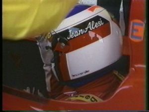
This time is the analysis of Ferrari F1 engine sound.
Driver is Jean Alesi.

![]() car3.wav (44.1kHz / Stereo / 6sec / 1,027KB)
car3.wav (44.1kHz / Stereo / 6sec / 1,027KB)
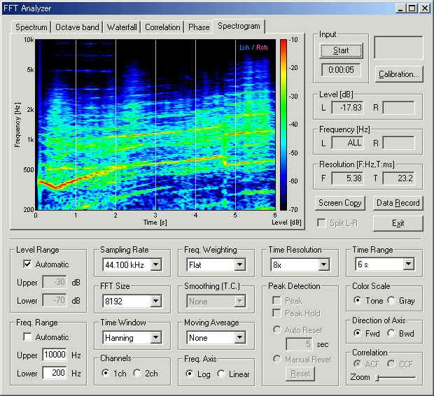
Same as last time, the wav file was loaded on the Recorder and analyzed by the FFT analyzer of the Realtime Analyzer of DSSF3.
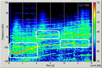
Below is the spectrogram of the engine sound. Sound energy at a given time and frequency is displayed by the color map. Red area indicates the strong frequency component contained in the sound. Very strong tonal components (red curves) can be seen throughout the recording. It corresponds to the listening impression, which is heard as high-pitched sharp sound. Pitch of the sound is increasing throughout the recording, meaning the engine speed is becoming higher and higher. Gear shift points can be found at around 0.5 s and 4.8 s, where the frequency drops rapidly and increases again.
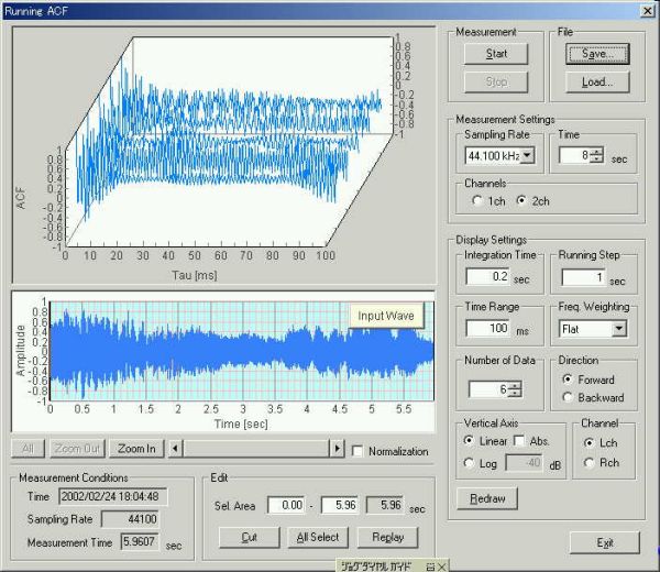
Next, the running ACF (Auto-Correlation Function) analysis was applied to the same sound. Running ACF is the time domain analysis that is capable of detecting the periodic events better than the frequency analysis. This is the reason why we apply this method to the analysis of sounds emitted from motor, car engine, and other equipments and machinery. Of course, the autocorrelation is a good analysis method for musical instruments and voices, because most sounds are periodic or quasi-periodic in nature.
Open the "Running ACF" window from the Realtime Analyzer, and load the wav file. Step by step instruction of the ACF analysis is here. Save data into the measurement database and analyze it by the Sound Analyzer (SA). See carf1.htm too.
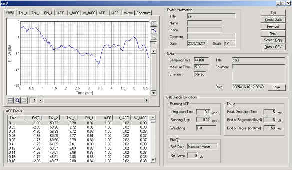
Sound file is loaded on the running ACF window. The bottom panel shows the sound waveform and the top panel shows the 3D display of the running ACF.
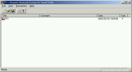
Data is saved, and analyzed by Sound Analyzer (SA). The data to be analyzes is listed in this display.
Calculation conditions were set as follows. Integration time (analysis data length) was set to 0.2 sec, and running step (calculation interval) was set to 0.02 sec. These values are comparable to those of the spectrogram (i.e. in the spectrogram, analysis data length is: FFT size (8192) / Sampling rate (44100) = 0.185 s, and calculation interval is Resolution [T]: 23.2 ms = 0.0232 s).
After the calculation is completed, analysis results are displayed in several graphs and tables of the acoustic parameters. Below (Phi(0)) is the time course of the change in the relative sound level.
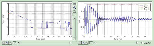
Next is the result of Tau_1 [ms], the delay time of the first peak in the ACF. Roughly speaking, it corresponds to the fundamental frequency shown in the spectrogram. Difference is that Tau_1 is represented in time, that is, 1000 / Tau_1 [ms]= Frequency [Hz]. For example, 10 ms of Tau_1 means the fundamental frequency of 100 Hz. So, the upside down of Tau_1 graph looks like the red curve in the spectrogram.
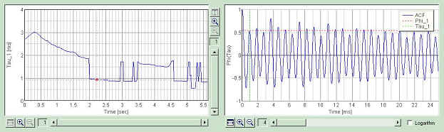
The ACF waveforms at several timings are shown below. Red mark in the time course of Tau_1 indicates the point of which ACF is shown.
The first is at 0.04 sec. The ACF has periodic peaks those are decreasing gradually. The first peak corresponds to the beginning of the red curve in the spectrogram (370 Hz).
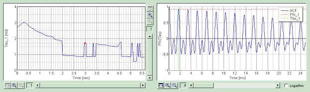
Second is at 2.2 sec. At this point, the first peak in the ACF is at 0.9 ms, corresponding to the frequency of 1100 Hz. Compare it to the spectrogram. Note that the second peak of the ACF (1.8 ms) is higher than the first peak. And the ACF has the periodic structure peaked at 3.6 ms. Those peaks corresponds to the frequency components at 540 Hz and 280 Hz.
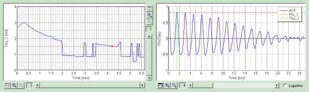
Third is at 3.0 sec. This time, the first peak shifts from 0.9 to 1.8 ms. This is the second peak in the above ACF. Relative heights of the peaks in the ACF may be decided by the balance of the harmonic components contained in the sound.
Fourth is at 4.2 sec. At this point, the peak around 1 ms disappears.
As we can see in the spectrogram, the first component (between 200 and 500 Hz) dominates from 0 to 2 seconds, then the second component (around at 1000 H) becomes stronger from 2 to 4 seconds. The first components dominates again from 4 seconds.
Finally, the ACF parameter Tau_e is shown. This value represents the degree of reverberation of sound. Comparing the result of Automobile noise analysis 2, this sound has much longer reverberation. Tau_e values of 50-100 ms are comparable to fast tempo orchestra music. It may be one reason of the liveness of this sound.
February 2002 by M. Sakurai