1. INTRODUCTION
For many years, environmental noise has been evaluated in terms of the
statistical sound pressure level (SPL), represented as Lx or
Leq, and its power spectrum measured by a
monaural sound level meter. The SPL and power spectrum alone, however, do
not provide a description that matches subjective evaluations of
environmental noise. Descriptions of many subjective attributes such as
preference and diffuseness, as well as primary sensations (loudness,
pitch, and timbre), can be based on a model of the response of the human
auditory-brain system to sound fields [1],
and the predictions of that model have been found to be consistent with
experimental results. The loudness of band-limited noise, for example, has
recently been shown to be affected by the effective duration of the
autocorrelation function (ACF), te,
as well as by the SPL [2, 3].
When a fundamental frequency of complex tones is below about 1200 Hz, the
pitch and its strength are indicated well by t1
and f1
respectively [4]. In particular,
the ACF factors obtained at (te)min
are good indicators of differences in the subjective evaluation of the
noise source and the noise field [5,
6].
The model consists of autocorrelators on
the signals at two auditory pathways and an interaural crosscorrelator
between then signals, and it takes into account the specialization of the
cerebral hemispheres in humans. The ACF and interaural crosscorrelation
function (IACF) of sound signals arriving at both ears are calculated.
Orthogonal factors F(0), te,
t1, and f1
are extracted from the ACF as described in detail in section 3 [7].
The factors LL, IACC, tIACC,
and WIACC are extracted from the IACF.
A software system that can obtain the ACF and IACF factors for any noise
sources has been developed [8],
and this paper describes the analytical process used to extract these
factors and also discusses the way they can be used to identify a noise
source.
2. OUTLINE OF THE MEASUREMENT SYSTEM
The measurement system consists of two microphones arranged as a binaural
pair, a laptop computer, and software that extracts the ACF and IACF factors
from real-time noise data. The system can measure environmental noise
automatically and simultaneously calculate the ACFs for the two signals and
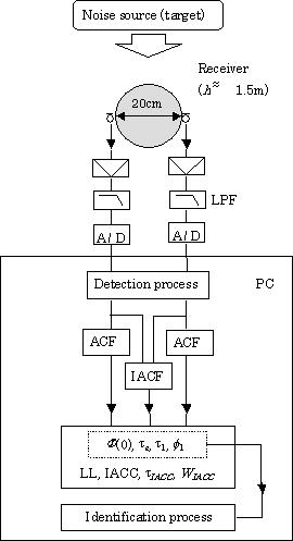
the IACF of the dual signal. Figure 1
is a flow chart of the method used to calculate the ACF and IACF factors.
FIGURE 1.
A flow chart of the
system for measuring environmental noise. ACF and IACF factors are extracted
through the process of automatic detection of the environmental noise
(target). The noise is identified by using four ACF factors. (LPF: low-pass
filter; PC: computational system.)
Dual-channel electrostatic microphones are used as the receiver, and a sphere between the microphones is used as a simple dummy head. Preliminary investigations comparing a human head, a dummy head, and a styrene foam sphere 20 cm in diameter revealed that the physical factors discussed here are not much affected by the shape of the head. The sampling frequency is usually 44.1 kHz and all the orthogonal factors are extracted from the ACF and IACF in real time. The noise source may then be identified by the use of ACF factors as described in section 4. The IACF factors mainly indicate the spatial information like the directivity or diffuseness in relation to the noise source. For further information for other aspects on the system, refer to our web site [9].
3. CALCULATION OF ORTHOGONAL FACTORS
3.1. PEAK-DETECTION OF ENVIRONMENTAL NOISE
A number of measurement sessions of the
environmental noise to be analyzed are extracted by a peak-detection
process. In order to automatically extract environmental noises or target
noises from a continuous noise, a monoaural energy
Fll(0)
or
Frr(0),
which is energy at the left or the right ear entrance, respectively, is
continuously analyzed. The peak-detection procedure is shown in Figure 2,
and the conditions determined in this analysis are listed in Table
1.
FIGURE 2.
Procedure
for extracting target noise for a single session. The concept of running
integration interval is also presented. Running ACF and running IACF are
conducted for every sessions to extract physical factors.
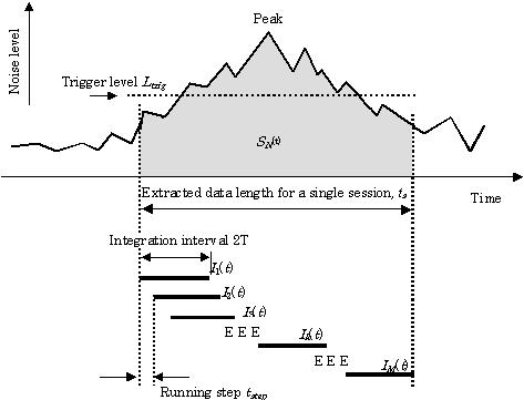
TABLE 1
Conditions to be determined in the detection process, the calculation
of the running ACF and running IACF, and the extraction of te
|
|
|
| Calculation process | Conditions |
|
|
|
| (a) Detection process | Trigger level Ltrig
(dB) Data length for a single session ts(s) |
| (b) Calculation of running ACF and running IACF | Integration interval 2T(s) Running step tstep (ms) |
| (c) Calculation of te | Time interval for detecting peaks Dt (ms) |
|
|
|
The interval for the
calculation of F(0)
can be fairly long, say 1 s, when the noise is a continuous one such as
aircraft noise or railway noise, but a shorter interval must be used when
the noise is brief or intermittent. For the running calculation in equation
(1) described below, however, it may be necessary to select an interval
longer than the integration interval. Thus, this time interval must be
determined according to the kind of the noise source. This enables F(0)
to be determined more accurately than it can be
determined when using a normal sound level meter with a long time constant.
The peaks cannot be detected unless the trigger level Ltrig
is properly set in advance. The appropriate Ltrig value
also varies according to the kind of target noise, the distances between the
target and the receiver, and atmospheric conditions. It must therefore be
determined by means of a preliminary measurement. It is easy to determine
the value of Ltrig, when the distance between the target
and the receiver is short and there is no interfering noise source near the
receiver. The noise centered on its maximum F(0)
is recorded on the system as a single session. The duration of one session
for each target noise, ts, should be selected so as to include
F(0)
peak after exceeding Ltrig
value. For normal environmental noise like aircraft noise
and railway noise, the value of ts
can be about 10 s. This is different from steady state
noise with longer duration or intermittent noise with shorter duration. Note
that the present system cannot be used when there are interfering noises. As
shown in Figure 2, the set of sessions {S1(t),
S2(t), S3(t), ..., SN(t);
N: the number of sessions, 0 < t< ts}
are stored on the system automatically.
The running ACF and running
IACF for each session SN(t) with duration ts
are analyzed as shown in the figure. Here we consider only a single session
in order to explain the process of "running". Appropriate values
for the integration interval 2T and running step tstep
are determined before the calculation. As explained in reference [6],
the recommended integration interval seems to be around 30 (te)min,
where (te)min
is the minimum value of the running series of values te,
and can easily be found by preliminary measurement. This is found by the use
of data of different kinds of environmental noises. In most cases, adjoining
integration intervals overlap each other. The ACF and the IACF are
calculated for every step (n = 1, 2, ..., M) within one
session with the range of 2T which shifts in every tstep,
as {(0, 2T), (tstep, tstep + 2T),
(2tstep, 2tstep + 2T),..., ((M
– 1)tstep, (M – 1)tstep
+ 2T)}. Physical factors are extracted from each step of the ACF and
the IACF. Note that 2T must be sufficiently longer than the expected
value of te.
Also, it should be deeply related to an "auditory time-window" for
sensation of each step. A 2T between 0.1 and 0.5 s may be appropriate
for environmental noise [5],
but a value near 2.5 s is recommended for music [6].
If 2T is less than this range, the (te)min
converges at a certain value. In most cases, the tstep is
recommended around 0.1 s. If a more detailed activity of fluctuation is
necessary, a shorter tstep should be selected.
As is well known, the ACF and the IACF are analyzed by
using the FFT for the binaural signals and then using the inverse FFT. The
A-weighting filter and frequency characteristics of microphones must be
taken into consideration after the process of FFT.
3.2. ACF FACTORS
The ACFs at the left and right ears are,
respectively, represented as
Fll
(t)
and Frr
(t).
In discrete numbers, they are represented as Fll(i)
and Frr(i)
(1 < i < Tf ; f
: sampling frequency (Hz); i : integer). In the calculation of F(0)
for left and right values, Fll(i)
and Frr(i)
are averaged as follows:
 . . |
(1) |
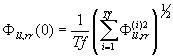
An accurate value for the SPL is given by
| SPL | ||
|
(2) |
where Fref(0) is the F(0) at the reference sound pressure, 20 mPa. The binaural listening level is the geometric mean of Fll(0) and Frr(0):
|
(3) |
Since this F(0)
is the denominator for normalization of the IACF, it can be considered to
be calssified as one of the IACF factors: or the right hemispheric spatial
factors [1].
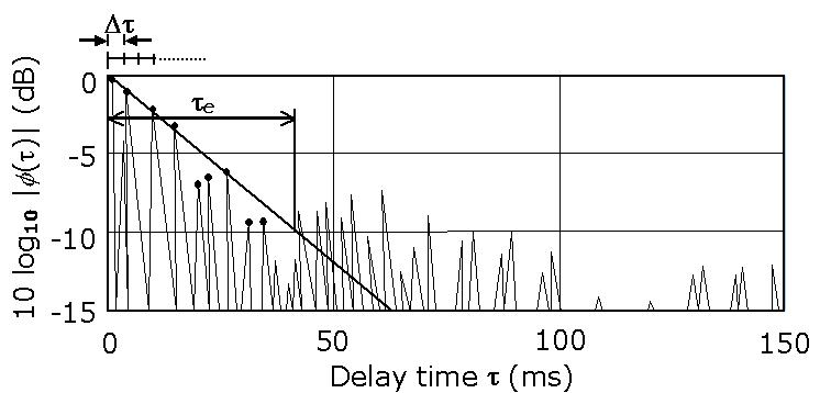
The effective duration,
te,
is defined by the delay time at which the envelope of the normalized ACF
becomes 0.1 (the 10 percentile delay: see Figure 3).
FIGURE 3.
An example of the calculation of
the effective duration, te,
from normalized ACF by linear fitting to the initial envelope of the ACF.
The normalized ACF for the left and right ears, fll,rr (t), is obtained as
|
(4) |
It is easy to obtain te
if the vertical axis is transformed into the decibel (logarithmic) scale,
because the linear decay for initial ACF is usually observed as shown in
the figure. For the linear regression, the least mean square (LMS) method
for ACF peaks which are obtained within each constant short time range Dt
is used. The Dt
is used for the detection of peaks in the ACF and must be carefully
determined before calculation. In calculating te,
the origin of the ACF ( = 0, at t
= 0) is sometimes excluded if it is not in the
regression line. As an extreme example, if the target noise consists of a
pure tone and a white noise, rapid attenuation at the origin due to the
white-noise components is observed, and the subsequent decay is kept flat
because of the pure-tone component. In such a case, the envelope function
of ACF must be figured out.
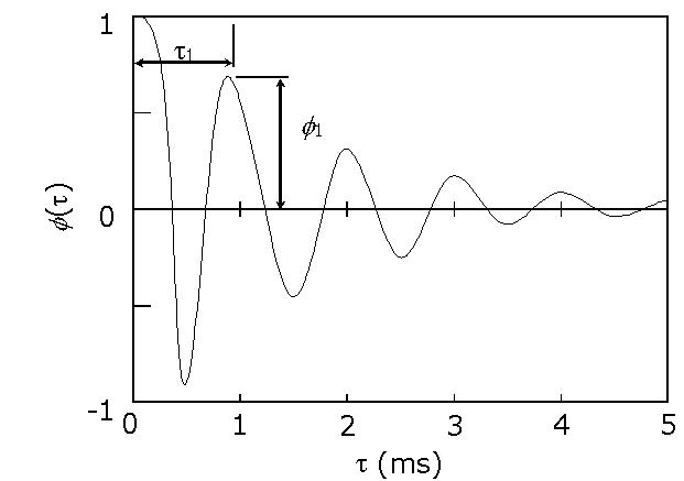
As shown in Figure 4, t1
and f1
are, respectively, the delay time and amplitude of the first peak of the
normalized ACF. The first maximum must be determined as a main peak
avoiding local minor peaks. The factors tn
and fn
(n > 2) are excluded because they
are usually related to t1
and f1.
FIGURE 4. Definitions of t1 and f1 for the normalized ACF.
3.3. IACF FACTORS
The IACF between sound signals at left and right ears is represented
as
Flr(t)
( - 1 < t
< + 1 (ms)). In the digital form, it is represented as Flr(i)
( - f /
103 < i < f
/ 103 ; i :
integer, where negative values signify the IACF as the left channel is
delayed). Thus, it is enough to consider only the range from - 1 to + 1
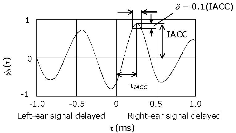
ms, which is the maximum possible delay between the ears. The IACC is a
factor related to the subjective diffuseness. As shown in Figure 5, it is
obtained as the maximum amplitude of the normalized IACF flr(i)
within the delay range.
FIGURE 5.
Definitions
of the IACC, tIACC,
and WIACC descriptors from the IACF.
Thus,
|
(5) |
The normalized IACF is given by
|
(6) |
The value of tIACC
is simply obtained at the time delay of the maximum amplitude. For example, if tIACC
is greater than zero (positive), the sound source is on the right side of the
receiver or is perceived as if it were. As shown in Figure 5, the value of WIACC
is given by the width of the peak at the level 0.1 (IACC) below the maximum
value. The coefficient 0.1 is approximately used as JND at IACC = 1.0.
The listening level LL is obtained by the manner represented in equation (2)
upon replacing SPL with LL.
Thus, physical factors extracted from fine structures of the ACF and IACF are
obtained for each integration interval as running values.
4. SOURCE IDENTIFICATION USING THE ACF FACTORS
As shown in Figure
1, noise sources are identified by using four ACF factors in the present stage.
Since the F(0) varies according to the distance between the source and receiver,
special attention is paid to the conditions for calculation if the distance is unknown.
Even if the factor F(0) is not useful,
the noise source can be identified by using the other three factors.
Remaining IACF factors may be taken into account if the spatial information is changed.
One of the guidelines to figure out the minimum te,
(te)min,
which represents the most active part of the noise signal,
is the fact that the piece is most deeply associated with subjective responses [10].
The distances between the values of each factor
at (te)min for the unknown target data
(indicated by the symbol a in equations (7-10),
and values for the template (indicated by the symbol b) are calculated.
Here, "target" is used as an environmental noise as an object to be identified by the system.
Template values of a set of typical ACF factors for a specific environmental noise are prepared,
and these templates for comparison with an unknown noise.
The distance D(x) (x: F(0), te,
t1,
and f1)
is calculated in the following manner:
|
(7) |
||
| |
(8) |
|
| |
(9) |
|
| |
(10) |
The total distance D of the target can be represented as the sum of the right-hand terms of equations (7)-(10), so
|
(11) |
where W(x) (x: F(0), te)min, t1, and f1) signifies the weighting coefficient. The template with the nearest D can be taken as the identified noise source. The method used to compute the weighting coefficients is described in Appendix A.
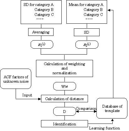
APPENDIX A: COMPUTATION OF THE WEIGHT COEFFICIENT
Weighting coefficients W(x) (x: F(0),
te, t1,
and f1) in equation (11)
are obtained by using statistical values s1(i) and s2(i).
As shown in Figure A1, s1(i) is the
arithmetic mean of the standard deviations (SD) for all categories of the ACF
factor. Here category means a set of data for the same kind of noise. s2(i)
is the SD of the arithmetic means for each category. Values of W(x)
are given as ![]() after
normalization by maximum values among factors
after
normalization by maximum values among factors ![]() .
This square root processing is experiential and would be improved by
introduction of a better function. The procedure is explained as follows. As a
factor with larger SD between noise sources and with smaller SD among a certain
source can distinguish the different kinds of noise, the weighting of such
factor should be larger than that of the other factors. If the learning function
toward the improvement of a template is given, a template is overwritten in
order by average values of each ACF factor between the latest session and the
previous data in the system.
.
This square root processing is experiential and would be improved by
introduction of a better function. The procedure is explained as follows. As a
factor with larger SD between noise sources and with smaller SD among a certain
source can distinguish the different kinds of noise, the weighting of such
factor should be larger than that of the other factors. If the learning function
toward the improvement of a template is given, a template is overwritten in
order by average values of each ACF factor between the latest session and the
previous data in the system.
FIGURE A1.
5. REMARKS
This paper described the detection of environmental noise, the analysis of
ACF and IACF factors, and a process for identifying unknown environmental
noises. The computational system described here may be useful for characterizing
environmental noises. Such a noise can be identified by using four factors
extracted from the ACF: F(0), te,
t1, and
f1.
Though the spatial factors extracted from the IACF (LL, IACC, tIACC,
and WIACC) are not used for the identification in this paper,
spatial information on the noise source including its degree of diffuseness and
its direction from the receiver can be described by these spatial factors.
Experimental results which include spatial factors from the IACF are
demonstrated in references [11, 12]
in this special issue.
ACKNOWLEDGMENTS
The authors would like to thank Mr. Shinichi Aizawa for his invaluable
assistance with programming the software. This work was supported by the
Research and Development Applying Advanced Computational Science and Technology
Program of the Japan Science and Technology Corporation (ACT-JST), 1999.
REFERENCES
| 1. | Y. ANDO 1998 Architectural Acoustics: Blending Sound Sources, Sound Fields, and Listeners. New York: A1P/Springer-Verlag. |
| 2. | I. G. N. MERTHAYASA and Y. ANDO 1996 Japan and Sweden Symposium on Medical Effects of Noise. Variation in the autocorrelation function of narrow band noises; their effect on loudness judgment. |
| 3. | S. SATO, H. SAKAI and Y. ANDO in Journal of Sound and Vibration. The loudness of "complex noise" in relation to the factors extracted from the autocorrelation function (to be published). |
| 4. | M. INOUE, Y. ANDO and T. TAGUTI in Journal of Sound and Vibration. The frequency range applicable to pitch identification based upon the autocorrelation function model (to be published). |
| 5. | K. MOURI, K. AKIYAMA and Y. ANDO in Journal of Sound and Vibration. Preliminary study on recommended time duration of source signals to be analyzed, in relation to its effective duration of autocorrelation function (to be published). |
| 6. | Y. ANDO, T. OKANO and Y. TAKEZOE 1989 The Journal of the Acoustical Society of America 86, 644-649. The running autocorrelation function of different music signals relating to preferred temporal parameters of sound fields. |
| 7. | Y. ANDO in Journal of Sound and Vibration. A theory of primary sensations measuring environmental noise (to be published). |
| 8. | M. SAKURAI, S. AIZAWA and Y. ANDO 1999 The Journal of the Acoustical Society of America 105, 1369. An internet-oriented system for acoustic measurements of sound fields. |
| 9. | Web site of Yoshimasa Electronic Inc. (URL: http://www.ymec.co.jp/index.htm). |
| 10. | K. MOURI, K. AKIYAMA and Y. ANDO 2000 Journal of Sound and Vibration 232, 139-147. Relationship between subjective preference and the alpha-brain wave in relation to the initial time delay gap with vocal music. |
| 11. | H. SAKAI, S. SATO, N. PRODI and R. POMPOLI in Journal of Sound and Vibration. Measurement of regional environmental noise by use of a PC-based system: an application to the noise near the airport 'G. Marconi' in Bologna (to be published). |
| 12. | K. FUJII, Y. SOETA and Y. ANDO in Journal of Sound and Vibration. Acoustical properties of aircraft noise measured by temporal and spatial factors (to be published). |